Free dashboards

We are offering free dashboards people ....... yeah you heard it right....!!

So what do I need to do to get one?.....

Okay here are the steps:
Step 1:
Send a mock up excel data sheet of yours (send it to exceldashboarder@gmail.com)

Step 2:
Tell us the metrics you would like to evaluate

Step 3:
We will go through your requirements and make a mock up dashboard!!

Dashboarder contacts you after feasibility is verified. After the design is finalized we cook your dashboard people.

We have a 90 day timeline.....after the design is finalized

So come on people , shoot.

Please note: This offer closes 1st july, 2014 :). Corporates will be preferred while selecting dashboard requests

Marketing Expense VBA Excel Dashboard

Loong time since last post....!


How have you been!!


Marketing Expense Dashboard helps in finding out the trends in the various marketing expenses that are incurred.


What will it support?

1. Trend Analysis by month
2. Sustainable data model

Here are some of the views of the dashboard

View 1:

View 2:

Let me know if this interests you......Beware Macro Inside ;)

Displaying more charts in an Excel worksheet using Indirect Function

Hey there!!

Today's task: Using a single Excel Sheet to fit more charts .Capacity Utilisation it is!



Key Concepts:

1. Indirect Function  :

Key Requirements:

• Lot of Excel Charts! for understanding the concept of conditional replacement

Charts Data Snapshot:

Charts Snapshot        :



These charts will be retrieved using Indirect function

Named Range used:

Steps for creating Dynamic Chart Switching with Radio Buttons

Note:First you will need two charts beforehand 

1. Inserting Option Buttons:

• Developer->Insert->Form Controls->Option Button
• Right click on Option Button , click on format control and input the following values

              

               Cell Link : $M$5 

       
               Named Range 'GetCharts' for conditional Chart switching

   2.  Insert a Picture from computer

   3. Click on the inserted picture

   4. After clicking,type " =GetCharts "in the formula bar    

  

   5.  After clicking enter the chart will be retrieved

Gentlemen!We have done it.Make best utilisation of available space in an excel sheet.Make it look more funky and an outlier !

Does it look like this?

Chart Views:

1.Radio Option Selected:   Graph 1

2.Option Selected:   Graph 2

Please comment with your email id for receiving the actual workbook

    

Using Camera tool in Excel 2010

Every come across a situation when you make a nice looking dashboard with lot of effort to impress your client/boss/any stake holder who can change things in your career and then you get a comment to shift the data table in the dashboard to somewhere else.Grrrrrrr.....very irritating huh .. after-all if some macro is populating your table you have to change code also !.

But then MS has made life easier with its camera tool.

What is camera  doing in my tools?

• Camera clicks a snap of the selected area on the excel spreadsheet and lets you place the image anywhere in the Excel Workbook.
• Now this snap is of those particular cells and hence any activity in these cells will be reflected in the picture taken by camera tool

Very useful in

• Making table positioning flexible in Excel Workbook
• To make charts uneditable by converting them into pictures

How do I add camera tool?

For Excel 2010 users

Step 1

Step 2

Step 3

Step 4

Step 5

Step 6

Using Camera tool:

1. Selected particular range in the excel worksheet and click on camera tool

      2.   Click on any cell in the worksheet and the picture representing selected range is displayed

Found this useful?..So go ahead and make some fantastic tables in Excel

Dynamic Excel Charts using Drop Down List

Hello Amigos,
Hope the day has been good so far!Why not make it awesome by learning something new?.

Lets us learn how to make Excel chart Axis labels and Series Values dynamically selected ,using drop down lists.Sounds refreshing ?Hell yeah!

Key Concepts:

1. Offset Function and  Named  Range  : Explained Earlier. Link=>
Offset and Named Range Concepts Background
2. Drop Down List

Key Requirements:

• Good 2 D data spread i.e Just another way of telling lot of data :D ,say Sales of ABC toy shop across different toy categories from January to December

Data Snapshot:

Named Range used:

1. Month_Data_Range : =OFFSET(Drop_Down_List_Test!$L$6,0,0,12,1)
2. Toy_Category_Sales_Data_Range : =OFFSET(Drop_Down_List_Test!$L$6,0,Drop_Down_List_Test!$A$4,12,1)

• Significance (Scroll_Bar_Test!$A$4): This input in the offset function shifts through various toy categories

Steps for creating Dynamic Chart with Drop Down List

1. Inserting Drop Down List (Also called Combo Box):

• Developer->Insert->Form Controls->Combo Box
• Right click on combo box , click on format control and input the following values

               Input range : $A$10:$A$17

               The range specifies distinct text values denoting toy categories

               Cell Link : $A$4  

              The toy category selected is reflected in the cell $A$4 which is then used by
               Named Range 'Toy_Category_Sales_Data_Range' for loading data of the relevant
               category

       

     Format Control Snapshot

    2.Insert a Bar chart

• Right click on the chart to select data
• Click on Add Legend Entries : 

         Series Name : Sales Value by Toy Category (whatever suits well ,no issues)  

         Series Values:Excel_Workbook_Name.xlsx!Named Range Name

         For Example:Series Value in the bar chart will be

         Dynamic_Dashboard.xlsx!Toy_Category_Sales_Data_Range

    3.Click on edit Horizontal Axis Labels for axis label data

        

         Axis Label Range: Excel_Workbook_Name.xlsx!Axis Named Range Name
         For example:Axis label range in the bar chart will be

         Dynamic_Dashboard.xlsx!Month_Data_Range

Clap Clap Calp! for yourself .Your done and how? .Now look smart and make some fantastic excel chart,leaving peers far behind

Oops forgot something in the appreciation mood!

Launch your creation with OK button click of Select Data Source of the chart

Chart Views:

1.Option Selected:   Games Toy Category

2.Option Selected:   Puzzles Toy Category

Please comment with your email id for receiving the actual workbook

    

Using Scroll Bar in Excel Charts

Aha! That eternal problem of accommodating lot of data in an Excel Chart.Lets just give it a little push in the right direction

Key Concepts:

1. Offset Function
2. Named Range
3. Scroll Bar

Requirements:

• Lots of data!

Let us zoom through them with an example

    1.Offset Function

Syntax : Offset(Reference,Row,Cols,[Height],[Width])

For Example:

Offset(E6,0,1,3,1)

In order of occurrence in the formula:

• E6: Referenced Cell.This Input specifies which is the starting point of data range.For example,In our case the cell with value "January".This is useful when we want to look quarter wise data with starting display month changing.Can be said to be the anchor for relative reference.

• 0:Number of rows to shift from the anchor cell.This option helps to shift data range on scroll bar change

• 1:Number of columns to shift from the anchor cell.

• 3:Number of row data to display. Example:We will display  quarter sales for a Toy Shop and hence 3 here specifies Data of 3 rows i.e 3 months

• 1: Number of column data to display. Example:We will display Sales column data

So what does the formula say finally,huh?

Get me data range which is starting from column beside the cell E6 i.e F6 and extending up to  data of 3 rows i.e F8.Hence the dynamic data range built is F6:F8.This shows sales data for first three months.

Now repeat the same for months range corresponding to range.The formula will minutely change and will be :Offset(E6,0,0,3,1)

    2.Named Range : Named Ranges help to encapsulate dynamic data reference.

      

     Prepare two named ranges

• Month_Data_Range :Formula=> Offset(E6,Scroll_Bar_Test!$A$2,0,3,1)
• Sales_Data_Range : Formula=> Offset(E6, Scroll_Bar_Test!$A$2 ,1,3,1)

  3.Scroll Bar:

• Insert a scroll bar from Developer->Insert->Form Controls->Scroll Bar
• Right click on Scroll Bar and click on Format Control
• In the cell link write $A$2.The cell value determines which month to display by shifting data from anchor cell by rows specified in the cell $A$2
• Also,put minimum value as 0 and maximum value as 10 in the format control tab of the scroll bar.This is because we want to display data from Jan(1 )to Dec(12) only.
• Maximum Value is 10 because in cell $A$2 it specifies to the offset formula to move data range from anchor by 10 rows and include 3 row data from $F$14 which brings the last data month to be viewed as December
• Incremental Change in format control of Scroll Bar means incremented $A$2 i.e cell linked to scroll bar by 3 when clicked on the scroll bar arrowheads.This is optional though!

Almost done!

Now, last but not the least lets insert a chart...say a bar chart for  proof of concept.

Steps 

1. Insert a bar chart
2. Right click on the chart to select data
3. Click on Add Legend Entries : 

• Series Name : Sales Value (whatever suits well ,no issues)  
• Series Values:Excel_Workbook_Name.xlsx!Named Range Name
• For Example:Series Value in the bar chart will be

          Dynamic_Dashboard.xlsx!Sales_Data_Range

     4.Click on edit Horizontal Axis Labels for axis label data

• Axis Label Range: Excel_Workbook_Name.xlsx!Axis Named Range Name
• For example:Axis label range in the bar chart will be

         Dynamic_Dashboard.xlsx!Month_Data_Range

Tryst with destiny!!! with a background of a heavy metal. Phew its done .

Launch your creation with OK button click of Select Data Source of the chart

         

Looks something like this?

And this on scroll bar change?

Please leave your email id in the comment box for me to send you the actual excel workbook.

Hyper Smash.

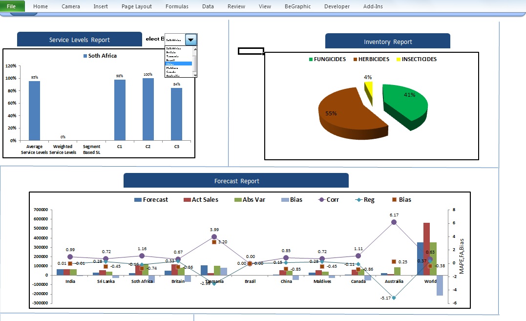
Excel Dynamic Dashboards BI simplified

With the breakthrough Excel power making BI for SME's an easier option.Let me show you one of the dynamic dashboards.This is first in series of many more powerful dashboards to come.Please leave your digital footprint as Email ID if you want to go through the actual dashboard which will be mailed to you.I am an avid excel worshipper.Excel has not only made my data analytic s easier but also lets me go home earlier.So all the dashboarders out there please review it and provide valuable feedback.


The Dashboard show above closely works with VBA and has total sustainable model.It loads its own data and also provides cleaning check.

Awaiting Inputs!!!